TL;DR: Generating stable RPCs is hard, and I'm not sure how to do it!
RPCs in the context of the geospatial world are equations for describing how a geometrically raw sensor image can be related to a location in the real world. RPC can variously expand to Rational Polynomial Coefficient or Rapid Positioning Coefficients. They consist of 80 coefficents for a ratio of two third degree polynomials (for x and y) plus 10 more values for normalizing image and geographic coordinates.
A couple background papers include one by Vincent Tao and others on Understanding the Rational Function Model (pdf), and one by Gene Dial and J. Grodecki titled RPC Replacement Camera Models (pdf). These date from the mid-2000s, but they reference some earlier work by Gene Dial and J. Grodecki who seem to have played the seminal role in promoting the use of RPCs as generic replacements for rigerous camera models. I believe the major satellite image vendors have now been delivering RPC models (example) for raw scenes for on the order of a decade.
I, and others, have added support to GDAL for reading and representing RPCs as metadata over the a number of years, as well as support for evaluating RPCs in gdalwarp as a way of georeferencing images. At it's very simplest a command like the following can be used to roughly rectify a raw image that has RPCs.
gdalwarp -rpc raw.tif rectified.tif
In fact, at FOSS4G NA this year, a command like this was the big reveal in Paul Morin's discussion of how the Polar Geospatial Center was able to efficiently process huge numbers of satellite scenes of the polar regions. I was rather surprised since I wasn't aware of this capability being in significant use. However the above use example will usually do a relatively poor job. RPCs encapsulate the perspective view of the satellite and as such you need to know the elevation of an early location in order to figure out exactly where it falls on the raw satellite image. If you had a relatively flat image at a known elevation you can specify a fixed elevation like this:
gdalwarp -rpc -to RPC_HEIGHT=257 raw.tif rectified.tif
However, in an area that is not so flat, you really need a reasonably could DEM (digital elevation model) of the region so that distortion effects from terrain can be taken into account. This is particularly important if the view point is relatively low (ie. for an airphoto) or if the image is oblique rather than nadir (straight down). You should be able to do this using a command referencing a DEM file for the area like this, though to be honest I haven't tried it recently (ever?) and I'm not sure how well it works:
gdalwarp -rpc -to RPC_DEM=srtm.tif raw.tif rectified.tif
The above is essentially review from my point of view. But with my recent move from Google to Planet Labs I have also become interested in how to generate RPCs given knowledge of a camera model, and the perspective view from a satellite. This would give us the opportunity to deliver raw satellite scenes with a generic description of the geometry that can already be exploited in a variety of software packages, including GDAL, OSSIM, Orfeo Toolbox and proprietary packages like ArcGIS, Imagine and PCI Geomatica. However, I had no idea how this would be accomplished and while I earned an Honours BMath, I have let the modest amount of math I mastered in the late 80's rot ever since.
So, using what I am good at, I started digging around the web for open source implementations for generating RPCs. Unfortunately, RPC is a very generic term much more frequently used to mean "Remote Procedure Call" in the software development world. Nevertheless, after digging I learned that the Orfeo Toolbox (OTB) has a program for generating RPCs from a set of GCPs (ground control points). Ground control points are just a list of locations on an image where the real world location is known. That is a list of information like (pixel x, pixel y, longitude, latitude, height). That was exciting, and a bit of digging uncovered the fact that in fact Orfeo Toolbox's RPC capability is really just a wrapper for services used from OSSIM. In particular core RPC "solver" is found in the source files ossimRpcSolver.cc, and ossimRpcSolver.h. They appear to have been authored by the very productive Garrett Potts.
Based on the example of the Orfeo Toolbox code, I wrote a gcps2rpc C++ program that called out to libossim to transform GCPs read from a text file into RPCs written to a GDAL VRT file.
For my first attempt I created 49 GCPs in a 7x7 pattern. The elevations were all zero (ie. they were on the WGS84 ellipsoids) and they were generated using custom code mapping from satellite image pixels to ground locations on the ellipsoid. I included simple code in gcps2rpc to do a forward and reverse evaluation of the ground control points to see how well they fit the RPC. In the case of this initial experiment the forward transformation, (long, lat, height) to (pixel, line) worked well with errors in the order of 1/1000th of a pixel. Errors in the inverse transformation, (pixel, line, height) to (long, lat) was less good with worst case errors on the order of 1/10th of a pixel.
At first I wasn't sure what to make of the errors in the inverse direction. 1/10th of a pixel wasn't terrible from my perspective, but it was still a fairly dramatic difference from the tiny errors in the forward direction. I tried comparing the results from evaluating the RPCs with OSSIM and with GDAL. To test with GDAL I just ran gdaltransform something like this.
gdaltransform -rpc -i simulated_rgb.vrt
-85.0495014028 39.7243133317 (entered in terminal)
2016.00011619623 1792.00003975369 0 (output in terminal)
and:
gdaltransform -rpc simulated_rgb.vrt
2016 1792 (entered in terminal)
-85.0495014329239 39.7243132735733 0 (output in terminal)
I found that GDAL and OSSIM agreed well in the forward transform, but while they both had roughly similar sized errors in the inverse they were still fairly distinct results. Reading through the code the reasoning became fairly obvious. They both use iterative solutions for the inverse transform and start with very different initial guesses, and they have fairly weak requirements for covergence. In the case of GDAL the convergence threshold was 1/10th of a pixel. OK, so that leaves me thinking there may be room to improve the inverse functions but accepting that the errors I'm seeing are really all about the iterative convergence.
Next I tried using the RPCs with gdalwarp to actually "rectify" the image. Initially I just left a default elevation of zero for gdalwarp, so I used a command like:
gdalwarp -rpc simulated_rgb.vrt ortho_0.tif
The results seemed plausible but I didn't have a particularly good way to validate it. My test scene is in Indiana, so I used a lat/long to height web service to determine that the region of my scene had a rough elevation of 254m above sea level (we will treat that as the same as the ellipsoid for now). So I tried:
gdalwarp -rpc -to RPC_HEIGHT=254 simulated_rgb.vrt ortho_254.tif
On review of the resulting image, it exactly overlayed the original. I had been hoping the result would have been slightly different based on the elevation. After a moments reflection and a review of the RPC which had many zero values in the terms related to elevation I realized I had't provided sufficient inputs to actually model the perspective transform. I had't given any GCPs at different heights. Also, the example code made it clear that an elevation sensitive RPC could not be generated with less than 80 GCPs (since the equations have 80 unknowns).
My next step was to produce more than 80 GCPs and to ensure that there was more than one elevation represented. It seemed like two layers of 49 GCPs - one at elevation zero, and one at an elevation of 300m should be enough to do the trick, so I updated my GCP generating script to produce an extra set with an ellipsoid that was 300m "bigger". I then ran that through gcps2rpc.
I was pleased to discover that I still got average and maximum errors at the GCPs very similar to the all-zero case. I also confirmed that the GCPs at 300m were actually at a non-trivially different location. So it seemed the RPCs were modelling the perspective view well, at least at the defining positions. I thought I was home free! So I ran a gcpwarp at a height of 0m, 300m and 254m. The results at 0m and 300m looked fine, but somehow the results at 254 meters was radically wrong - greatly inflated! A quick test with gdaltransform gave a sense of what was going wrong:
gdaltransform -rpc simulated_rgb.vrt
0 0 0
-85.036383862713 39.6431112403042 0
0 0 300
-85.0363998100256 39.6431575414329 300
0 0 254
-84.9815303476089 39.2011322215184 254
Essentially this showed that pixel/line location 0,0 was transforming reasonably at the elevations 0 and 300, but at 254 the results were far from the region expected. Clearly the RPCs were not generally modelling the perspective view well. This is the point I am at now. Is it not clear to me what I will need to do to produce stable RPCs for my perspective view from orbit. Perhaps there is a more suitable pattern or number of GCPs to produce. Perhaps the OSSIM RPC generation code needs to be revisited. Perhaps I need to manually construct RPC coefficients that model the perspective view instead of just depending on a least squares best fit to produce reasonable RPCs from a set of GCPs.
Anyways, I hope that this post will provide a bit of background on RPCs to others walking this road, and I hope to have an actually solution to post about in the future.
Showing posts with label gdal. Show all posts
Showing posts with label gdal. Show all posts
Sunday, September 8, 2013

Friday, February 18, 2011
MapServer TIFF Overview Performance
Last week Thomas Bonfort, MapServer polymath contacted me with some surprising performance results he was getting while comparing two ways of handling image overviews with MapServer.
In one case he had a single GeoTIFF file with overviews built by GDAL's gdaladdo utility in a separate .ovr file. Only one MapServer LAYER was used to refer to this image. In the second case he used a distinct TIFF file for each power-of-two overview level, and a distinct LAYER with minscale/maxscale settings for each file. So in the first case it was up to GDAL to select the optimum overview level out of a merged file, while in the second case MapServer decided which overview to use via the layer scale selection logic.
He was seeing performance using the MapServer multi-layer approach being about twice what it was with letting GDAL select the right overview. He prepared a graph and scripts with everything I needed to reproduce his results.
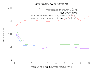
I was able to reproduce similar results at my end, and set to work trying to analyse what was going on. The scripts used apache-bench to run MapServer in it's usual cgi-bin incarnation. This is a typical use case, and in aggregate shows the performance. However, my usual technique for investigating performance bottlenecks is very low-tech. I do a long run demonstrating the issue in gdb, and hit cntl-c frequently, and use "where" to examine what is going on. If the bottleneck is dramatic enough this is usually informative. But I could not apply this to the very very short running cgi-bin processes.
So I set out to establish a similar work load in a single long running MapScript application. In doing so I discovered a few things. First, that there was no way to easily load the OWSRequest parameters from an url except through the QUERY_STRING environment variable. So I extended mapscript/swiginc/owsrequest.i to have a loadParamsFromURL() method. My test script then looked like:
The second thing I learned is that Thomas' recent work to directly use libjpeg and libpng for output in MapServer had not honoured the msIO_ IO redirection mechanism needed for the above. I fixed that too.
This gave me a proces that would run for a while and that I could debug with gdb. A sampling of "what is going on" showed that much of the time was being spent loading TIFF tags from directories - particularly the tile offset and tile size tag values.
The base file used is 130000 x 150000 pixels, and is internally broken up into nearly 900000 256x256 tiles. Any map request would only use a few tiles but the array of pointers to tiles and their sizes for just the base image amounted to approximately 14MB. So in order to get about 100K of imagery out of the files we were also reading at least 14MB of tile index/sizes.
The GDAL overview case was worse than the MapServer overview case because when opening the file GDAL scans through all the overview directories to identify what overviews are available. This means we have to load the tile offset/size values for all the overviews regardless of whether we will use them later. When the offset/size values are read to scan a directory they are subsequently discarded when the next directory is read. So in cases where we need to come back to a particular overview level we still have to reload the offsets and sizes.
For several years I have had some concerns about the efficiency of files with large tile offset/size arrays, and with the cost of jumping back and forth between different overviews with GDAL. This case highlighted the issue. It also suggested an obvious optimization - to avoid loading the tile offset and size values until we actually need them. If we access an image directory (ie overview level) to get general information about it such as the size, but we don't actually need imagery we could completely skip reading the offsets and sizes.
So I set about implementing this in libtiff. It is helpful being a core maintainer of libtiff as well as GDAL and Mapserver. :-) The change was a bit messy, and also it seemed a bit risky due to how libtiff handled directory tags. So I treat the change as as an experimental (default off) build time option controlled by the new libtiff configure option --enable-defer-strile-load.
With the change in place, I now get comparable results using the two different overview strategies. Yipee! Pleased with this result I have commited the changes in libtiff CVS head, and pulled them downstream into the "built in" copy of libtiff in GDAL.
However, it occurs to me that there is still an unfortunate amount of work being done to load the tile offset/size vectors when doing full resolution image accesses for MapServer. A format that computed the tile offset and size instead of storing all the offsets and sizes explicitly might do noticeable better for this use case. In fact, Erdas Imagine (with a .ige spill file) is such a format. Perhaps tonight I can compare to that and contemplate a specialized form of uncompressed TIFF files which doesn't need to store and load the tile offset/sizes.
I would like to thank Thomas Bonfort for identifying this issue, and providing such an easy to use set of scripts to reproduce and demonstrate the problem. I would also like to thank MapGears and USACE for supporting my time on this and other MapServer raster problems.
In one case he had a single GeoTIFF file with overviews built by GDAL's gdaladdo utility in a separate .ovr file. Only one MapServer LAYER was used to refer to this image. In the second case he used a distinct TIFF file for each power-of-two overview level, and a distinct LAYER with minscale/maxscale settings for each file. So in the first case it was up to GDAL to select the optimum overview level out of a merged file, while in the second case MapServer decided which overview to use via the layer scale selection logic.
He was seeing performance using the MapServer multi-layer approach being about twice what it was with letting GDAL select the right overview. He prepared a graph and scripts with everything I needed to reproduce his results.

I was able to reproduce similar results at my end, and set to work trying to analyse what was going on. The scripts used apache-bench to run MapServer in it's usual cgi-bin incarnation. This is a typical use case, and in aggregate shows the performance. However, my usual technique for investigating performance bottlenecks is very low-tech. I do a long run demonstrating the issue in gdb, and hit cntl-c frequently, and use "where" to examine what is going on. If the bottleneck is dramatic enough this is usually informative. But I could not apply this to the very very short running cgi-bin processes.
So I set out to establish a similar work load in a single long running MapScript application. In doing so I discovered a few things. First, that there was no way to easily load the OWSRequest parameters from an url except through the QUERY_STRING environment variable. So I extended mapscript/swiginc/owsrequest.i to have a loadParamsFromURL() method. My test script then looked like:
import mapscript

map = mapscript.mapObj( 'cnes.map')
mapscript.msIO_installStdoutToBuffer()

for i in range(1000):
  req = mapscript.OWSRequest()
  req.loadParamsFromURL( 'LAYERS=truemarble-gdal&FORMAT=image/jpeg&SERVICE=WMS&VERSION=1.1.1&REQUEST=GetMap&STYLES=&EXCEPTIONS=application/vnd.ogc.se_inimage&SRS=EPSG%3A900913&BBOX=1663269.7343875,1203424.5723063,1673053.6740063,1213208.511925&WIDTH=256&HEIGHT=256')
  map.OWSDispatch( req )
The second thing I learned is that Thomas' recent work to directly use libjpeg and libpng for output in MapServer had not honoured the msIO_ IO redirection mechanism needed for the above. I fixed that too.
This gave me a proces that would run for a while and that I could debug with gdb. A sampling of "what is going on" showed that much of the time was being spent loading TIFF tags from directories - particularly the tile offset and tile size tag values.
The base file used is 130000 x 150000 pixels, and is internally broken up into nearly 900000 256x256 tiles. Any map request would only use a few tiles but the array of pointers to tiles and their sizes for just the base image amounted to approximately 14MB. So in order to get about 100K of imagery out of the files we were also reading at least 14MB of tile index/sizes.
The GDAL overview case was worse than the MapServer overview case because when opening the file GDAL scans through all the overview directories to identify what overviews are available. This means we have to load the tile offset/size values for all the overviews regardless of whether we will use them later. When the offset/size values are read to scan a directory they are subsequently discarded when the next directory is read. So in cases where we need to come back to a particular overview level we still have to reload the offsets and sizes.
For several years I have had some concerns about the efficiency of files with large tile offset/size arrays, and with the cost of jumping back and forth between different overviews with GDAL. This case highlighted the issue. It also suggested an obvious optimization - to avoid loading the tile offset and size values until we actually need them. If we access an image directory (ie overview level) to get general information about it such as the size, but we don't actually need imagery we could completely skip reading the offsets and sizes.
So I set about implementing this in libtiff. It is helpful being a core maintainer of libtiff as well as GDAL and Mapserver. :-) The change was a bit messy, and also it seemed a bit risky due to how libtiff handled directory tags. So I treat the change as as an experimental (default off) build time option controlled by the new libtiff configure option --enable-defer-strile-load.
With the change in place, I now get comparable results using the two different overview strategies. Yipee! Pleased with this result I have commited the changes in libtiff CVS head, and pulled them downstream into the "built in" copy of libtiff in GDAL.
However, it occurs to me that there is still an unfortunate amount of work being done to load the tile offset/size vectors when doing full resolution image accesses for MapServer. A format that computed the tile offset and size instead of storing all the offsets and sizes explicitly might do noticeable better for this use case. In fact, Erdas Imagine (with a .ige spill file) is such a format. Perhaps tonight I can compare to that and contemplate a specialized form of uncompressed TIFF files which doesn't need to store and load the tile offset/sizes.
I would like to thank Thomas Bonfort for identifying this issue, and providing such an easy to use set of scripts to reproduce and demonstrate the problem. I would also like to thank MapGears and USACE for supporting my time on this and other MapServer raster problems.
Sunday, July 18, 2010
OGR DXF Upgrade
Well, I just finished up a week of work implementing PCIDSK Vector write and update support. My next task is an upgrade to the OGR DXF driver requested by Stadt Uster to better meet their production requirements.
They need the ability to control layer naming, production of dash patterns, and producing objects as block references.
Currently the DXF writer is dependent on everything except the entities section coming directly from a template file. This has meant it was not practical to create layers, line styles and block references on the fly. This is going to have to change now, though we will continue to use the template header extensively.
The first approach considered was just to require the user to develop a template header with all the layer names, line styles and block references predefined. This might have been adequate for Uster who have specific needs and once a template was prepared they could generally just reuse it for additional products. But it would have made the new capabilities of very little utility to other users of GDAL.
So the planned approach has two parts. First we scan the template header for layer definitions, and block definitions (and possibly line style definitions). Then as we go through the entities if we find these layers or blocks referenced we just use them directly.
However, if we find layers referenced from the objects being written to the DXF file (based on the "Layer" attribute) we will automatically create a new layer in the header, matching the configuration of the default layer ("0"). This means we can automatically create layers that have identity even if they are otherwise indistinguishable.
For block references we use a roughly similar approach. We prescan for block definitions, but then we extend them with any entities written to an OGR layer named "Blocks". Normally all DXF entities are exposed through an OGR layer called "entities" though when writing we accept any layer name, except now for Blocks which is special. Then when we write we allow these blocks to be referenced based on a BlockName attribute.
Corresponding behavior will also be available when reading. If desired (a config option turned on) we will expose block definitions as a Blocks layer, and the actual block references in the entities layer will just be a point feature with insertion information. The default behavior will remain what it does not - which is to inline copies of the block geometries for each block reference as this is the only approach that will be handled gracefully by most applications or writers.
For line styles it is not clear that it is helpful to predefine them (though I'll examine that during implementation). The only aspect we are interested in preserving and producing is dash-dot patterns. But while writing I will create new line styles for each such pattern encountered, and then write them out to the header.
Currently the DXF writer copies the template header to the output file, then writes entities, then appends the trailer template. In the future I will need to write the entities to a temporary file, storing up block, layer and line style definitions in memory. Then on closing the dataset I will need to compose the full header, append the entities and trailer.
I dislike this pattern. It introduces a need for temporary files which can lead to surprising disk use requirements. Also, if something goes wrong the temp files may not get cleaned up properly. We also lose any hope of streaming operation. However, to achieve what we want to with the DXF driver it seems unavoidable.
Hopefully I'll have the DXF changes in trunk within a couple weeks. If there are folks interested in DXF generation, keep an eye on SVN for updates. Beta testers appreciated!
They need the ability to control layer naming, production of dash patterns, and producing objects as block references.
Currently the DXF writer is dependent on everything except the entities section coming directly from a template file. This has meant it was not practical to create layers, line styles and block references on the fly. This is going to have to change now, though we will continue to use the template header extensively.
The first approach considered was just to require the user to develop a template header with all the layer names, line styles and block references predefined. This might have been adequate for Uster who have specific needs and once a template was prepared they could generally just reuse it for additional products. But it would have made the new capabilities of very little utility to other users of GDAL.
So the planned approach has two parts. First we scan the template header for layer definitions, and block definitions (and possibly line style definitions). Then as we go through the entities if we find these layers or blocks referenced we just use them directly.
However, if we find layers referenced from the objects being written to the DXF file (based on the "Layer" attribute) we will automatically create a new layer in the header, matching the configuration of the default layer ("0"). This means we can automatically create layers that have identity even if they are otherwise indistinguishable.
For block references we use a roughly similar approach. We prescan for block definitions, but then we extend them with any entities written to an OGR layer named "Blocks". Normally all DXF entities are exposed through an OGR layer called "entities" though when writing we accept any layer name, except now for Blocks which is special. Then when we write we allow these blocks to be referenced based on a BlockName attribute.
Corresponding behavior will also be available when reading. If desired (a config option turned on) we will expose block definitions as a Blocks layer, and the actual block references in the entities layer will just be a point feature with insertion information. The default behavior will remain what it does not - which is to inline copies of the block geometries for each block reference as this is the only approach that will be handled gracefully by most applications or writers.
For line styles it is not clear that it is helpful to predefine them (though I'll examine that during implementation). The only aspect we are interested in preserving and producing is dash-dot patterns. But while writing I will create new line styles for each such pattern encountered, and then write them out to the header.
Currently the DXF writer copies the template header to the output file, then writes entities, then appends the trailer template. In the future I will need to write the entities to a temporary file, storing up block, layer and line style definitions in memory. Then on closing the dataset I will need to compose the full header, append the entities and trailer.
I dislike this pattern. It introduces a need for temporary files which can lead to surprising disk use requirements. Also, if something goes wrong the temp files may not get cleaned up properly. We also lose any hope of streaming operation. However, to achieve what we want to with the DXF driver it seems unavoidable.
Hopefully I'll have the DXF changes in trunk within a couple weeks. If there are folks interested in DXF generation, keep an eye on SVN for updates. Beta testers appreciated!
Sunday, March 14, 2010
Slaying the Datum Shift Dragon
In the last few weeks, I believe I have made substantial improvements to the way datum shift information is derived from the EPSG dictionary for use in GDAL/OGR, PROJ.4 and related packages.
The EPSG database model supports having multiple datum shift options for a particular datum, such as "Potsdam Rauenberg 1950 DHDN" to get to WGS84. This reflects the reality that datum conversion is often an approximation for which there may be multiple reasonable solutions. Often different datum shift parameters are appropriate depending on the sub-region of the datum being used.
Many other coordinate system dictionary models and GIS systems do *not* provide for a multiplicity of datum shift options. For instance, the OGC Well Known Text representation of a coordinate system only allows for one TOWGS84[] clause indicating the preferred mapping to WGS84. This is also true of many software packages, including those based on PROJ.4 and it's epsg based dictionary.
In the past, the code I had implemented for translating the epsg database to a dictionary format assumed that datum shift parameters should only be carried into the dictionary if there was one, and only one shift available in the EPSG database. I took this approach because it seemed very dangerous to arbitrarily select one of several possible datum shifts without any intrinsic knowledge about which was most appropriate. I depending on users seeing that no datum shift was available in the default translation and taking this to mean that they had to do some research to establish what was most appropriate for them.
Predictably, the real result was massive confusion and complaints. At one time if there was no datum shift available, PROJ.4 would just do a transformation based on the change of ellipsoid which was often a very poor choice. So in PROJ 4.6.0 I altered the code not attempt any datum shift transformation if either or both of the source and destination coordinate system lacked datum shift information.
While this got rid of one family of errors, it also triggered lots of additional frustration and confusion. Part of this was just because there was a change of behavior. But it was also pushing people a bit harder to determine the appropriate datum shift and they did not like having to do this.
So, at last, I have taken the plunge and reworked the scripts used to translate the EPSG dictionary so that they attempt to pick one shift if there are several available. I follow a few heuristics in this effort.
1) I discard any datum shifts marked as deprecated.
2) I examine the supersession table to identify any datum shifts that have been superceeded by newer forms and ignore the superceeded forms.
3) I try to pick the datum shift with the larges "area of use" region under the assumption that it will likely be the broad use shift rather than a shift only applicable in a small area.
4) I examine the datum_shift_pref.csv file to see if there is a user supplied preferred datum shift to use. If so, I use that.
The result of all this is a datum_shift.csv file which includes all the datum shifts, with one of them marked as preferred. That preferred version goes into the gcs.csv file for use with the associated geographic coordinate system.
This seems to be working reasonable well, and I did a big pass through open tickets in GDAL, libgeotiff and PROJ.4 to find outstanding datum shift issues. I believe that the bulk are now resolved.
Currently GDAL, and the PROJ.4 dictionary are just using the preferred datum shift. But the intention of keeping the datum_shift.csv file with all the possible shifts for any given GCS is that savvy applications could let the user choose. Also, my hope is that an each mechanism will be added in the future so that users can alter the preferred setting in the datum_shift.csv file, and then have the gcs.csv regenerated. That waits to be done.
I'm also fixing a few other issues in the coordinate system realm including support for axis orientation (ie. South Orientated Transverse Mercator) and fixing a few other translations. I'd like to thank INGRES who have supported this work as part of an effort to bring top notch coordinate system support into the INGRES geospatial project. I'd also like to thank Jan Hartmann, and Mikael Rittri who assisted with suggested approaches, and verification of the results.
The EPSG database model supports having multiple datum shift options for a particular datum, such as "Potsdam Rauenberg 1950 DHDN" to get to WGS84. This reflects the reality that datum conversion is often an approximation for which there may be multiple reasonable solutions. Often different datum shift parameters are appropriate depending on the sub-region of the datum being used.
Many other coordinate system dictionary models and GIS systems do *not* provide for a multiplicity of datum shift options. For instance, the OGC Well Known Text representation of a coordinate system only allows for one TOWGS84[] clause indicating the preferred mapping to WGS84. This is also true of many software packages, including those based on PROJ.4 and it's epsg based dictionary.
In the past, the code I had implemented for translating the epsg database to a dictionary format assumed that datum shift parameters should only be carried into the dictionary if there was one, and only one shift available in the EPSG database. I took this approach because it seemed very dangerous to arbitrarily select one of several possible datum shifts without any intrinsic knowledge about which was most appropriate. I depending on users seeing that no datum shift was available in the default translation and taking this to mean that they had to do some research to establish what was most appropriate for them.
Predictably, the real result was massive confusion and complaints. At one time if there was no datum shift available, PROJ.4 would just do a transformation based on the change of ellipsoid which was often a very poor choice. So in PROJ 4.6.0 I altered the code not attempt any datum shift transformation if either or both of the source and destination coordinate system lacked datum shift information.
While this got rid of one family of errors, it also triggered lots of additional frustration and confusion. Part of this was just because there was a change of behavior. But it was also pushing people a bit harder to determine the appropriate datum shift and they did not like having to do this.
So, at last, I have taken the plunge and reworked the scripts used to translate the EPSG dictionary so that they attempt to pick one shift if there are several available. I follow a few heuristics in this effort.
1) I discard any datum shifts marked as deprecated.
2) I examine the supersession table to identify any datum shifts that have been superceeded by newer forms and ignore the superceeded forms.
3) I try to pick the datum shift with the larges "area of use" region under the assumption that it will likely be the broad use shift rather than a shift only applicable in a small area.
4) I examine the datum_shift_pref.csv file to see if there is a user supplied preferred datum shift to use. If so, I use that.
The result of all this is a datum_shift.csv file which includes all the datum shifts, with one of them marked as preferred. That preferred version goes into the gcs.csv file for use with the associated geographic coordinate system.
This seems to be working reasonable well, and I did a big pass through open tickets in GDAL, libgeotiff and PROJ.4 to find outstanding datum shift issues. I believe that the bulk are now resolved.
Currently GDAL, and the PROJ.4 dictionary are just using the preferred datum shift. But the intention of keeping the datum_shift.csv file with all the possible shifts for any given GCS is that savvy applications could let the user choose. Also, my hope is that an each mechanism will be added in the future so that users can alter the preferred setting in the datum_shift.csv file, and then have the gcs.csv regenerated. That waits to be done.
I'm also fixing a few other issues in the coordinate system realm including support for axis orientation (ie. South Orientated Transverse Mercator) and fixing a few other translations. I'd like to thank INGRES who have supported this work as part of an effort to bring top notch coordinate system support into the INGRES geospatial project. I'd also like to thank Jan Hartmann, and Mikael Rittri who assisted with suggested approaches, and verification of the results.
Wednesday, February 10, 2010
GDAL 1.7.0 is dead, long live GDAL 1.7.1
Due to a serious bug in GDAL 1.7.0 resulting in all Erdas Imagine files produced by the release being unreadable to any non-GDAL applications, including Erdas Imagine, the project has decided to retract the 1.7.0 release. In it's place today we have issued a GDAL/OGR 1.7.1 release. I sincerely hope that use of 1.7.0 in the wild will not end up producing unreadable Erdas Imagine files that haunt us for years.
The introduction of the bug was due to a very subtle issue, and it didn't affect GDAL's ability to read the files. So our extensive regression tests for this file format did not detect any problems. But the lesson would appear to be that we still need mechanisms to do cross testing with other packages as often as possible. We are looking into ways of more vigorous and organized cross testing at major releases.
The introduction of the bug was due to a very subtle issue, and it didn't affect GDAL's ability to read the files. So our extensive regression tests for this file format did not detect any problems. But the lesson would appear to be that we still need mechanisms to do cross testing with other packages as often as possible. We are looking into ways of more vigorous and organized cross testing at major releases.
Monday, January 4, 2010
hsv_merge.py
Recently Trent Hare indicated an interest in an extension to the gdaldem program to produce a color relief image mixed with a hillshade.
The gdaldem utility is a utility program for producing various products from DEMs (elevation models). It was originally written by Matthew Perry, with contributions by Even Rouault, Howard Butler, and Chris Yesson to incorporate it into GDAL proper. It can produce color relief maps, hillshades, slope, aspect and various roughness values.
But what Trent wanted was a product with both a hillshade and a color relief image merged. The color relief shows overall elevation with color, and the hillshade gives a sense of local structure. He has been doing this with ImageMagick to produce the product from the hillshade and relief produced by gdaldem, but this resulted in the georeferencing being lost. It is accomplished by transforming the relief image to HSV (hue, saturation and value) color space, and then replacing the "value" portion with the hillshade greyscale image. The value is really the intensity or brightness. This is a common technique and is often used to merge high resolution greyscale imagery with lower resolution RGB image to produce a result with meaningful color and high resolution.
I reviewed the gdaldem.cpp code with the thought of adding a new mode, but it turns out the program is fairly complicated and a new hillshade/relief mode would likely be hard to maintain properly. So instead I set out to create a utility that could do the rgb/greyscale merge in hsv space as a standalone utility. When possible I prefer to do non-core utilities as python instead of C++. It feels lighter and easier for folks to munge for other purposes.
In Python we generally try to do image processing using the Python numpy package, so that is what I set out to do. For some things numpy lets us treat arrays as if they were scalars, and operate on the whole array with a single statement. So the "scalar" function to convert hsv to rgb looks like:
I was able to change this into a numpy based function that looked fairly similar in parts, but somewhat different in other areas:
The first step just breaks a single hsv array into three component arrays and is just bookkeeping:
The next few statements look very much like the original and are essentially simple math that happens to be done on whole arrays instead of single values. The only odd part is using "astype(int)" to convert to int instead of the int() builtin function that was used for scalars.
But following this there are many if/then else statements which had looked like:
Unfortunately we can't really do something quite like an if statement with numpy that will be evaluated on a per-pixel (array entry) basis. The old scalar logic assumed that if a condition was met, it could do something for that case, and return. But for arrays we are going to have to do things quite differently. The above is essentially a case statement, so we instead use the numpy choose() function like this:
The choose function goes through each entry in the "i" array, and uses it's value as an index into the set of possible return values (v,q,p,p,t,v in the first case). So if i[0] is 0, then the first item v[0] is assigned to r[0]. If i[0] was 4 then t[0] would be assigned to r[0]. Thus the six if statements are handled as a choose() with six possible return results, and the choose is evaluated for each array entry (pixel).
This works reasonably well for this very structured case. We then finish by merging the red, green and blue values into an 3 band array:
One thing missing in my rendition of this function is the saturation == 0 case:
It is very difficult to have the pixels for which the saturation is zero handled differently than all the rest since we can't actually return control to the caller for only some pixels (array entries). In this particular situation it seems that this was just an optimization and if s is zero the result will be v,v,v anyways so I just omitted this statement.
But this helps highlight the difficulty of taking different logic paths for different entries in the array using numpy. The rgb_to_hsv() logic was even more involved. The original was:
This became:
The key mechanism here is the computation of true/value masks (maxc_is_r, maxc_is_g, maxc_is_b) which are used with choose() statements to overlay different results on the pixels that match particular conditions. It may not be immediately evident, but we are essentially evaluating all the equations for all pixels even though the values are only going to be used for some of them. Quite wasteful.
The final result, hsv_merge.py, works nicely but I am once again left frustrated with the unnatural handling of logic paths in numpy. It took me over three hours to construct this small script. Most of that time was spent poring over the numpy reference trying to figure out how to do things that are dead easy in scalar python.
I love Python, but to be honest I still can't say the same for numpy.
The gdaldem utility is a utility program for producing various products from DEMs (elevation models). It was originally written by Matthew Perry, with contributions by Even Rouault, Howard Butler, and Chris Yesson to incorporate it into GDAL proper. It can produce color relief maps, hillshades, slope, aspect and various roughness values.
But what Trent wanted was a product with both a hillshade and a color relief image merged. The color relief shows overall elevation with color, and the hillshade gives a sense of local structure. He has been doing this with ImageMagick to produce the product from the hillshade and relief produced by gdaldem, but this resulted in the georeferencing being lost. It is accomplished by transforming the relief image to HSV (hue, saturation and value) color space, and then replacing the "value" portion with the hillshade greyscale image. The value is really the intensity or brightness. This is a common technique and is often used to merge high resolution greyscale imagery with lower resolution RGB image to produce a result with meaningful color and high resolution.
I reviewed the gdaldem.cpp code with the thought of adding a new mode, but it turns out the program is fairly complicated and a new hillshade/relief mode would likely be hard to maintain properly. So instead I set out to create a utility that could do the rgb/greyscale merge in hsv space as a standalone utility. When possible I prefer to do non-core utilities as python instead of C++. It feels lighter and easier for folks to munge for other purposes.
In Python we generally try to do image processing using the Python numpy package, so that is what I set out to do. For some things numpy lets us treat arrays as if they were scalars, and operate on the whole array with a single statement. So the "scalar" function to convert hsv to rgb looks like:
def hsv_to_rgb(h, s, v):
   if s == 0.0: return v, v, v
   i = int(h*6.0) # XXX assume int() truncates!
   f = (h*6.0) - i
   p = v*(1.0 - s)
   q = v*(1.0 - s*f)
   t = v*(1.0 - s*(1.0-f))
   if i%6 == 0: return v, t, p
   if i == 1: return q, v, p
   if i == 2: return p, v, t
   if i == 3: return p, q, v
   if i == 4: return t, p, v
   if i == 5: return v, p, q
   # Cannot get here
I was able to change this into a numpy based function that looked fairly similar in parts, but somewhat different in other areas:
def hsv_to_rgb( hsv ):

  h = hsv[0]
  s = hsv[1]
  v = hsv[2]

  i = (h*6.0).astype(int)
  f = (h*6.0) - i
  p = v*(1.0 - s)
  q = v*(1.0 - s*f)
  t = v*(1.0 - s*(1.0-f))

  r = i.choose( v, q, p, p, t, v )
  g = i.choose( t, v, v, q, p, p )
  b = i.choose( p, p, t, v, v, q )

  rgb = numpy.asarray([r,g,b]).astype(numpy.byte)

  return rgb
The first step just breaks a single hsv array into three component arrays and is just bookkeeping:
  h = hsv[0]
  s = hsv[1]
  v = hsv[2]
The next few statements look very much like the original and are essentially simple math that happens to be done on whole arrays instead of single values. The only odd part is using "astype(int)" to convert to int instead of the int() builtin function that was used for scalars.
  i = (h*6.0).astype(int)
  f = (h*6.0) - i
  p = v*(1.0 - s)
  q = v*(1.0 - s*f)
  t = v*(1.0 - s*(1.0-f))
But following this there are many if/then else statements which had looked like:
  if i%6 == 0: return v, t, p
  if i == 1: return q, v, p
  if i == 2: return p, v, t
  if i == 3: return p, q, v
  if i == 4: return t, p, v
  if i == 5: return v, p, q
Unfortunately we can't really do something quite like an if statement with numpy that will be evaluated on a per-pixel (array entry) basis. The old scalar logic assumed that if a condition was met, it could do something for that case, and return. But for arrays we are going to have to do things quite differently. The above is essentially a case statement, so we instead use the numpy choose() function like this:
  r = i.choose( v, q, p, p, t, v )
  g = i.choose( t, v, v, q, p, p )
  b = i.choose( p, p, t, v, v, q )
The choose function goes through each entry in the "i" array, and uses it's value as an index into the set of possible return values (v,q,p,p,t,v in the first case). So if i[0] is 0, then the first item v[0] is assigned to r[0]. If i[0] was 4 then t[0] would be assigned to r[0]. Thus the six if statements are handled as a choose() with six possible return results, and the choose is evaluated for each array entry (pixel).
This works reasonably well for this very structured case. We then finish by merging the red, green and blue values into an 3 band array:
rgb = numpy.asarray([r,g,b]).astype(numpy.byte)
One thing missing in my rendition of this function is the saturation == 0 case:
if s == 0.0: return v, v, v
It is very difficult to have the pixels for which the saturation is zero handled differently than all the rest since we can't actually return control to the caller for only some pixels (array entries). In this particular situation it seems that this was just an optimization and if s is zero the result will be v,v,v anyways so I just omitted this statement.
But this helps highlight the difficulty of taking different logic paths for different entries in the array using numpy. The rgb_to_hsv() logic was even more involved. The original was:
def rgb_to_hsv(r, g, b):
  maxc = max(r, g, b)
  minc = min(r, g, b)
  v = maxc
  if minc == maxc: return 0.0, 0.0, v
  s = (maxc-minc) / maxc
  rc = (maxc-r) / (maxc-minc)
  gc = (maxc-g) / (maxc-minc)
  bc = (maxc-b) / (maxc-minc)
  if r == maxc: h = bc-gc
  elif g == maxc: h = 2.0+rc-bc
  else: h = 4.0+gc-rc
  h = (h/6.0) % 1.0
  return h, s, v
This became:
def rgb_to_hsv( rgb ):

  r = rgb[0]
  g = rgb[1]
  b = rgb[2]

  maxc = numpy.maximum(r,numpy.maximum(g,b))
  minc = numpy.minimum(r,numpy.minimum(g,b))

  v = maxc

  minc_eq_maxc = numpy.equal(minc,maxc)

  # compute the difference, but reset zeros to ones to avoid divide by zeros later.
  ones = numpy.ones((r.shape[0],r.shape[1]))
  maxc_minus_minc = numpy.choose( minc_eq_maxc, (ones, maxc-minc) )

  s = (maxc-minc) / numpy.maximum(ones,maxc)
  rc = (maxc-r) / maxc_minus_minc
  gc = (maxc-g) / maxc_minus_minc
  bc = (maxc-b) / maxc_minus_minc

  maxc_is_r = numpy.equal(maxc,r)
  maxc_is_g = numpy.equal(maxc,g)
  maxc_is_b = numpy.equal(maxc,b)

  h = numpy.zeros((r.shape[0],r.shape[1]))
  h = numpy.choose( maxc_is_b, (h,4.0+gc-rc) )
  h = numpy.choose( maxc_is_g, (h,2.0+rc-bc) )
  h = numpy.choose( maxc_is_r, (h,bc-gc) )

  h = numpy.mod(h/6.0,1.0)

  hsv = numpy.asarray([h,s,v])

  return hsv
The key mechanism here is the computation of true/value masks (maxc_is_r, maxc_is_g, maxc_is_b) which are used with choose() statements to overlay different results on the pixels that match particular conditions. It may not be immediately evident, but we are essentially evaluating all the equations for all pixels even though the values are only going to be used for some of them. Quite wasteful.
The final result, hsv_merge.py, works nicely but I am once again left frustrated with the unnatural handling of logic paths in numpy. It took me over three hours to construct this small script. Most of that time was spent poring over the numpy reference trying to figure out how to do things that are dead easy in scalar python.
I love Python, but to be honest I still can't say the same for numpy.
Tuesday, December 15, 2009
Death by Complexity
This post will be incomprehensible.
Over the last three days I have spent 4.5 hours working on GDAL Ticket 3276 related to a failure to use external overviews with JPEG2000 compressed NITF files - in particular for NITF files containing more than one jpeg2000 image.
This bug was particularly hairy because it comes at the intersection of several things that are messy/complex in GDAL:
It turns out that .aux.xml metadata was supported for NITF subdatasets, and it was possible to build overviews for nitf subdatasets, and it was possible to substitute external tiff overviews for jpeg2000 data streams in an NITF file. But it was not possible to substitute external tiff overviews for jpeg2000 data stream in an nitf file with multiple images (subdatasets).
It took me a long time to figure out what aspects were broken, and how the various components were supposed to work even though I had implemented most of them. The problem is that many of these capabilities are rarely used, don't fit the standard GDAL model well, and were individually quite complex to implement. The complexity as the various aspects come together is compounded.
Each of the capabilities was added for fairly good reasons - mostly in order to provide a seamless, and performant user experience for GDAL users. But in order to provide this consistent external set of behaviors we are having to build more and more complexity into parts of GDAL - to the point where I am not sure it is sustainable.
Interestingly, most of this complexity has grown without input from the broader GDAL community. The PAM mechanism predated the modern Project Steering Committee and it's RFC process. I added the changes for PAM on subdatasets, and some of the specific NITF driver capabilities without discussion with the PSC on the assumption that they are either bug fixes, or are sufficiently driver-local that the PSC does not need to be involved. Possibly if these changes had needed to be justified in public, push back on the complexity might have prevented some.
The specific problem itself was fixed, as is documented in the ticket, with changeset 18312 holding the core fix. However, this fix is (IMHO) just adding additional fragility to the existing house of cards.
I don't really have a solution to the growing complexity, but perhaps thinking about, and starting to open up the issues a bit is a first step to containing the danger. There is certainly a cautionary tale or two in here.
BTW, GDAL 1.7.0Beta 1 is now released - testing and bug reports are welcome!
Over the last three days I have spent 4.5 hours working on GDAL Ticket 3276 related to a failure to use external overviews with JPEG2000 compressed NITF files - in particular for NITF files containing more than one jpeg2000 image.
This bug was particularly hairy because it comes at the intersection of several things that are messy/complex in GDAL:
- JPEG2000 in NITF is implemented by creating JP2KAK driver dataset wrapping the jpeg2000 image data within the NITF file, and then using it's bands indirectly as bands for the NITF dataset. These band objects still mostly think of the jpeg2000 dataset as "their" dataset but for some purposes we really might wish they knew about the NITF dataset that appears to own them.
- NITF files can contain more than one image. Such multi-image files are treated as containing subdatasets, one per image. For the most part these subdatasets are intended to act as freestanding things, but they are also, to some extent related back to the single file on disk containing the subdatasets.
- Overviews in GDAL are mostly handled through an overview manager object embedded in the GDALDataset base class. However, JPEG2000 images have built-in overviews not handled through the overview manager.
- The PAM (Persistant Auxilary Metadata) mechanism is used via an intermediate GDALPamDataset class to provide a way of storing additional information about datasets that the intrinsic format does not support. This information is stored in an .aux.xml file associated with the main data file.
- In GDAL 1.7 a new capability was added to store PAM information for subdatasets in an .aux.xml file associated with the main data file so that subdatasets would work as much like a regular dataset as possible.
- In GDAL 1.7 support was added for building overviews on subdatsets. Since normally overviews would be stored in a .ovr file with the same basename as the main filename, it was necessary to do something special so that overviews of subdataset would have one .ovr file per subdataset. This was accomplished by keeping the overview file name in the .aux.xml file associated with the subdataset.
It turns out that .aux.xml metadata was supported for NITF subdatasets, and it was possible to build overviews for nitf subdatasets, and it was possible to substitute external tiff overviews for jpeg2000 data streams in an NITF file. But it was not possible to substitute external tiff overviews for jpeg2000 data stream in an nitf file with multiple images (subdatasets).
It took me a long time to figure out what aspects were broken, and how the various components were supposed to work even though I had implemented most of them. The problem is that many of these capabilities are rarely used, don't fit the standard GDAL model well, and were individually quite complex to implement. The complexity as the various aspects come together is compounded.
Each of the capabilities was added for fairly good reasons - mostly in order to provide a seamless, and performant user experience for GDAL users. But in order to provide this consistent external set of behaviors we are having to build more and more complexity into parts of GDAL - to the point where I am not sure it is sustainable.
Interestingly, most of this complexity has grown without input from the broader GDAL community. The PAM mechanism predated the modern Project Steering Committee and it's RFC process. I added the changes for PAM on subdatasets, and some of the specific NITF driver capabilities without discussion with the PSC on the assumption that they are either bug fixes, or are sufficiently driver-local that the PSC does not need to be involved. Possibly if these changes had needed to be justified in public, push back on the complexity might have prevented some.
The specific problem itself was fixed, as is documented in the ticket, with changeset 18312 holding the core fix. However, this fix is (IMHO) just adding additional fragility to the existing house of cards.
I don't really have a solution to the growing complexity, but perhaps thinking about, and starting to open up the issues a bit is a first step to containing the danger. There is certainly a cautionary tale or two in here.
BTW, GDAL 1.7.0Beta 1 is now released - testing and bug reports are welcome!
Saturday, December 5, 2009
OGR DXF Driver
The last couple weeks I have been working on an OGR DXF driver. AutoCAD DXF format is a popular interchange format for CAD data, and to a somewhat lesser extent for goespatial map data often originating from engineering departments. It is a rather ugly format. Even though it is ASCII it is less than fun for humans to scan.
The raw machinery of the format is published by Autodesk, and lots of translators have been written for it in the past. However, I find it very frustrating that the format specifications fail to address the semantics of the format to any meaningful degree. It is assumed, I guess, that the person reading them is already deeply familiar with the AutoCAD data model.
So, for instance, it talks about the BLOCKS section, and the INSERT entity, but it never really explains that by defining a bunch of entities as a block, and then putting them into the drawing it makes it possible to treat a bunch of entities as a group. This has to be deduced. I have an old dxf file produced by FME that uses this as a mechanism to group a set of polylines that form a multipolygon, but I'm not sure how widely this approach is used.
In my driver, I have implemented two mechanisms for supporting blocks. In the case of non-text entities I try to accumulate the geometries I derive from the entities in the block into one OGC geometrycollection. But I also found that blocks in some drawings are used to group sets of text elements. In this case if I only use the geometries, I've discarded the important component - the text - so I collect the text entities as full features. And when I encounter the INSERT entity I push the original set of features into the input stream.
I spent most of a day implementing read support for the DIMENSION entity. This is essentially supposed to be a single object that shows a measurement on a drawing. The red part below is a single dimension element as rendered by QCAD.

Of course, there is no clear analog to this in OGR. So I ended up creating a single feature with a MULTILINESTRING geometry for the leaders, and arrows, and then pushed the label as a separate point feature with a LABEL style string.
I have made some effort to capture the drawing style information so that features can, in theory, be drawn similarly to AutoCAD by OGR applications. There is still really only one way to do this in OGR and that is to provide styling information as OGR Feature Style strings. This is a format that Daniel Morissette, myself and I believe Stephane Villeneuve defined many years ago as based closely on the sorts of styling supported by the mapinfo format(s). A few extensions have been made over the years, and a few OGR drivers utilize it to return styling information including DGN, and MapInfo. Andrey Kiselev has also done some stuff with it, so I presume there is a driver of his that uses it. So far the only two application that I know of using the feature style information are OpenEV and MapServer (via OGR autostyling).
I'm quite conflicted about the OGR feature style specification. I just hate to define "yet another" way of describing feature styling that is not closely related to any proper standard. I can't help but think there ought to be something more standards oriented to use as a basis. Perhaps OGC SLD, or SVG or something like that. But SLD didn't exist when we started, and does not express a lot of what I want. I don't really know that much about SVG - perhaps it would be a good choice. So, lacking a clear plan each time I need styling I do a bit more work on the OGR feature style specification while remaining less than fully committed to it as a long term thing.
Another aspect that was challenging was all the curves. I added the OGRGeometryFactory::approximateArcAngles() method as a generic mechanism to approximate arcs on an ellipsoid or circle as linestrings. The code was adapted from the Oracle driver and similar code exists in the DGN, and NTF drivers too I believe. So, finally this moves into the core.
One of the DXF curve types is a spline. Review the QCAD source code I found they implemented the spline rendering using rationale b-spline curves derived from Chapter 4 of An Introduction to NURBS by David Rogers. They release under the GPL so I can't directly use the code from QCAD without also putting GDAL/OGR under GPL restrictions, so I contacted the original author for permission to publish this code under the MIT/X license, like GDAL. He has indicated he has received my email and is considering the request ... so I wait.
In addition to the specification, I have also found the QCAD (and it's underlying dxflib library) to be a useful reference. I considered using dxflib but it really does not seem to solve any of the hard parts for me, and it would have added a dependency on an external library - complicating building of GDAL/OGR. The other very helpful resource was the v.in.dxf code from GRASS. This is a slightly less sophisticated dxf reader than OGR (IMHO) but it provided a very easy to understand implementation of a DXF reader for GIS data that was especially helpful in writing the proposal for the DXF driver. I also used it as a reference when implementing some of the element translations.
Before closing, I would like to thank Andreas Neumann and the City of Uster who have provided funding for this development. It seems that local government in Switzerland punches above it's weight in the free gis software world (the Kanton of Solothurn is also a big supporter of qgis, and related technologies as I understand). If only one in ten cities in the world made serious use of free gis software and provided enough financial support for one core developer it would have a huge boosting effect.
Anyways, preliminary DXF read support is in GDAL SVN now. Consider trying it out and providing feedbac.
The raw machinery of the format is published by Autodesk, and lots of translators have been written for it in the past. However, I find it very frustrating that the format specifications fail to address the semantics of the format to any meaningful degree. It is assumed, I guess, that the person reading them is already deeply familiar with the AutoCAD data model.
So, for instance, it talks about the BLOCKS section, and the INSERT entity, but it never really explains that by defining a bunch of entities as a block, and then putting them into the drawing it makes it possible to treat a bunch of entities as a group. This has to be deduced. I have an old dxf file produced by FME that uses this as a mechanism to group a set of polylines that form a multipolygon, but I'm not sure how widely this approach is used.
In my driver, I have implemented two mechanisms for supporting blocks. In the case of non-text entities I try to accumulate the geometries I derive from the entities in the block into one OGC geometrycollection. But I also found that blocks in some drawings are used to group sets of text elements. In this case if I only use the geometries, I've discarded the important component - the text - so I collect the text entities as full features. And when I encounter the INSERT entity I push the original set of features into the input stream.
I spent most of a day implementing read support for the DIMENSION entity. This is essentially supposed to be a single object that shows a measurement on a drawing. The red part below is a single dimension element as rendered by QCAD.

Of course, there is no clear analog to this in OGR. So I ended up creating a single feature with a MULTILINESTRING geometry for the leaders, and arrows, and then pushed the label as a separate point feature with a LABEL style string.
I have made some effort to capture the drawing style information so that features can, in theory, be drawn similarly to AutoCAD by OGR applications. There is still really only one way to do this in OGR and that is to provide styling information as OGR Feature Style strings. This is a format that Daniel Morissette, myself and I believe Stephane Villeneuve defined many years ago as based closely on the sorts of styling supported by the mapinfo format(s). A few extensions have been made over the years, and a few OGR drivers utilize it to return styling information including DGN, and MapInfo. Andrey Kiselev has also done some stuff with it, so I presume there is a driver of his that uses it. So far the only two application that I know of using the feature style information are OpenEV and MapServer (via OGR autostyling).
I'm quite conflicted about the OGR feature style specification. I just hate to define "yet another" way of describing feature styling that is not closely related to any proper standard. I can't help but think there ought to be something more standards oriented to use as a basis. Perhaps OGC SLD, or SVG or something like that. But SLD didn't exist when we started, and does not express a lot of what I want. I don't really know that much about SVG - perhaps it would be a good choice. So, lacking a clear plan each time I need styling I do a bit more work on the OGR feature style specification while remaining less than fully committed to it as a long term thing.
Another aspect that was challenging was all the curves. I added the OGRGeometryFactory::approximateArcAngles() method as a generic mechanism to approximate arcs on an ellipsoid or circle as linestrings. The code was adapted from the Oracle driver and similar code exists in the DGN, and NTF drivers too I believe. So, finally this moves into the core.
One of the DXF curve types is a spline. Review the QCAD source code I found they implemented the spline rendering using rationale b-spline curves derived from Chapter 4 of An Introduction to NURBS by David Rogers. They release under the GPL so I can't directly use the code from QCAD without also putting GDAL/OGR under GPL restrictions, so I contacted the original author for permission to publish this code under the MIT/X license, like GDAL. He has indicated he has received my email and is considering the request ... so I wait.
In addition to the specification, I have also found the QCAD (and it's underlying dxflib library) to be a useful reference. I considered using dxflib but it really does not seem to solve any of the hard parts for me, and it would have added a dependency on an external library - complicating building of GDAL/OGR. The other very helpful resource was the v.in.dxf code from GRASS. This is a slightly less sophisticated dxf reader than OGR (IMHO) but it provided a very easy to understand implementation of a DXF reader for GIS data that was especially helpful in writing the proposal for the DXF driver. I also used it as a reference when implementing some of the element translations.
Before closing, I would like to thank Andreas Neumann and the City of Uster who have provided funding for this development. It seems that local government in Switzerland punches above it's weight in the free gis software world (the Kanton of Solothurn is also a big supporter of qgis, and related technologies as I understand). If only one in ten cities in the world made serious use of free gis software and provided enough financial support for one core developer it would have a huge boosting effect.
Anyways, preliminary DXF read support is in GDAL SVN now. Consider trying it out and providing feedbac.
Subscribe to:
Posts (Atom)